MATLAB Eigenvalues and Eigenvectors

1. Understanding Eigenvalues and Eigenvectors
2. How to Find Eigenvalues and Eigenvectors in MATLAB Using the eig() Function
3. How to Find the Dominant Eigenvalue and Eigenvector in MATLAB Using the Power Iteration Method
4. How to Find the Eigenvector of a Specific Eigenvalue in MATLAB Using Inverse Iteration
5. Conclusion

Eigenvalues and eigenvectors play a fundamental role in various mathematical and engineering applications, including solving systems of linear equations, stability analysis, image processing, and machine learning. MATLAB provides powerful tools for computing eigenvalues and eigenvectors of matrices efficiently.

In this article, we will explore how to find eigenvalues and eigenvectors of a given matrix in MATLAB.

Understanding Eigenvalues and Eigenvectors

Before delving into the MATLAB implementation, let’s briefly review what eigenvalues and eigenvectors are.

Eigenvalues are scalar values that represent the scaling factor of the eigenvectors when a linear transformation is applied. Mathematically, for a square matrix ( A ), if ( \lambda ) is an eigenvalue of ( A ), and ( \mathbf{v} ) is the corresponding eigenvector, then ( A\mathbf{v} = \lambda\mathbf{v} ).

Eigenvectors are non-zero vectors that remain in the same direction after a linear transformation. They are associated with eigenvalues and play a crucial role in understanding the behavior of linear transformations.

How to Find Eigenvalues and Eigenvectors in MATLAB Using the eig() Function

In MATLAB, computing eigenvalues and eigenvectors of a matrix is made easy with the eig() function. This function is specifically used to find the eigenvalues and eigenvectors of a given square matrix.

Here are the syntax variations of the eig() function in MATLAB, along with its parameters:

e = eig(A)
[V,D] = eig(A)
[V,D,W] = eig(A)
e = eig(A,B)
[V,D] = eig(A,B)
[V,D,W] = eig(A,B)
[___] = eig(A,balanceOption)
[___] = eig(A,B,algorithm)
[___] = eig(___,outputForm)

Parameters:

• A: Input square matrix.
• B: (Optional) Another square matrix used for generalized eigenvalue problems.
• balanceOption: (Optional) Specifies whether to enable or disable balancing ("balance" or "nobalance").
• algorithm: (Optional) Specifies the algorithm to be used for computing generalized eigenvalues ("chol" or "qz").
• outputForm: (Optional) Specifies the output form for eigenvalues ("vector" or "matrix").
• e: Column vector containing eigenvalues.
• V: Matrix whose columns are right eigenvectors.
• D: Diagonal matrix containing eigenvalues.
• W: Matrix whose columns are left eigenvectors.

Behind the scenes, MATLAB’s eig() function employs sophisticated numerical algorithms to compute the eigenvalues and eigenvectors of a matrix. It often relies on iterative methods and matrix decompositions to achieve accurate results efficiently.

These algorithms are optimized to handle a wide range of matrix sizes and properties, ensuring robust performance across various applications.

Example 1: Basic Usage

Let’s start with a basic example. We’ll create a simple 2x2 matrix and use eig() to find its eigenvalues.

% Define the matrix
Matrix = [1 3; 4 2];

% Find eigenvalues
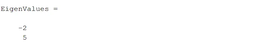
[EigenValues] = eig(Matrix)

In this example, we start by defining a 2x2 matrix named Matrix. This matrix serves as our input for finding its eigenvalues.

We call the eig() function with Matrix as the argument, and the function returns the eigenvalues, which are stored in the variable EigenValues. In MATLAB, eigenvalues are typically represented as a column vector.

Output:

Example 2: Finding Eigenvalues and Eigenvectors

Next, let’s find both the eigenvalues and eigenvectors of a matrix. We’ll reuse the same matrix as in Example 1.

% Define the matrix
Matrix = [1 3; 4 2];

% Find eigenvalues and eigenvectors
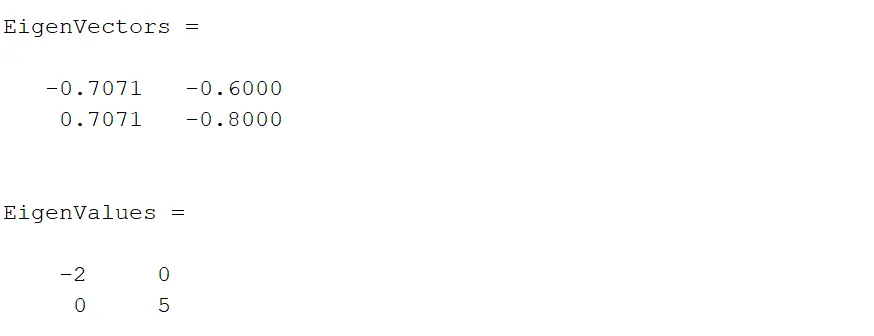
[EigenVectors, EigenValues] = eig(Matrix)

Again, we define our matrix Matrix, but this time we use a separate variable, EigenVectors, to store the computed eigenvectors. By calling eig() with Matrix, the function returns both the eigenvalues and eigenvectors.

The eigenvectors are organized as columns in the matrix EigenVectors, while the eigenvalues are stored in a diagonal matrix EigenValues. This provides a more comprehensive understanding of the matrix’s behavior under transformation.

Output:

Example 3: Sorting Eigenvalues

In real-world applications, it’s often useful to have eigenvalues sorted in ascending or descending order. We can achieve this by sorting the diagonal elements of the matrix returned by eig().

% Define the matrix
Matrix = magic(3);

% Find eigenvalues
[EigenVectors, EigenValues] = eig(Matrix);

% Sort eigenvalues
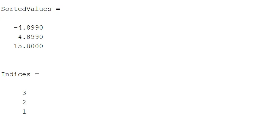
[SortedValues, Indices] = sort(diag(EigenValues))

In this example, we demonstrate how to achieve this sorting.

We start by defining our matrix Matrix using MATLAB’s magic() function, which generates a magic square matrix. Then, we use eig() to find the eigenvalues and store them in EigenValues.

To sort these eigenvalues, we extract the diagonal elements of EigenValues using the diag() function and sort them using MATLAB’s sort() function. This gives us the sorted eigenvalues in ascending order, along with the corresponding indices of the original order.

Output:

Example 4: Sorting Eigenvectors

Similarly, we can sort the eigenvectors corresponding to the sorted eigenvalues obtained in Example 3.

% Define the matrix
Matrix = magic(3);

% Find eigenvalues and eigenvectors
[EigenVectors, EigenValues] = eig(Matrix);

% Sort eigenvalues
[SortedValues, Indices] = sort(diag(EigenValues));

% Sort eigenvectors
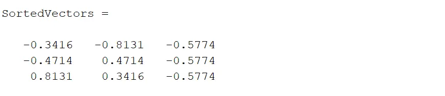
SortedVectors = EigenVectors(:, Indices)

Building upon the previous example, we extend our sorting to include eigenvectors. After finding the eigenvalues and eigenvectors of Matrix using eig(), we sort the eigenvalues as we did in Example 3.

Then, we use the obtained indices to rearrange the columns of EigenVectors accordingly, ensuring that the eigenvectors are sorted according to their eigenvalues. This ensures consistency between eigenvalues and eigenvectors, facilitating easier analysis and interpretation of the results.

Output:

Example 5: Generalized Eigenvalues and Eigenvectors

In some cases, we may need to find the generalized eigenvalues and eigenvectors of two matrices. This scenario arises in problems like stability analysis and control systems.

Here, we illustrate how to use eig() to compute the generalized eigenvalues and eigenvectors.

% Define the matrices
Matrix1 = magic(2);
Matrix2 = [1 2; 2 1];

% Find generalized eigenvalues and eigenvectors
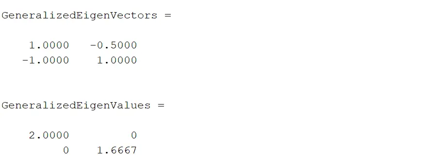
[GeneralizedEigenVectors, GeneralizedEigenValues] = eig(Matrix1, Matrix2)

In this example, we have two matrices, Matrix1 and Matrix2. We call eig() with both matrices as arguments.

The function returns the generalized eigenvalues in GeneralizedEigenValues and the corresponding eigenvectors in GeneralizedEigenVectors. These generalized eigenvalues and eigenvectors represent the solution to the equation Matrix1 * x = lambda * Matrix2 * x, where x is the eigenvector and lambda is the eigenvalue.

Output:

Example 6: Finding Eigenvalues, Right Eigenvectors, and Left Eigenvectors

MATLAB’s eig() function allows us to find not only the eigenvalues and right eigenvectors but also the left eigenvectors of a matrix. This capability allows us to thoroughly analyze the behavior of the matrix under both left and right transformations.

Let’s explore how to utilize this feature:

% Define the matrix
Matrix = magic(3);

% Find eigenvalues, right eigenvectors, and left eigenvectors
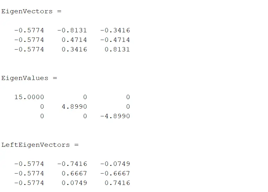
[EigenVectors, EigenValues, LeftEigenVectors] = eig(Matrix)

In this example, eig() returns three outputs: EigenVectors containing the right eigenvectors, EigenValues containing the eigenvalues, and LeftEigenVectors containing the left eigenvectors. Right eigenvectors satisfy the equation Matrix * EigenVectors = EigenVectors * EigenValues, while the left eigenvectors satisfy the equation LeftEigenVectors * Matrix = EigenValues * LeftEigenVectors.

These results provide a comprehensive understanding of the behavior and dynamics of the matrix under different transformations.

Output:

How to Find the Dominant Eigenvalue and Eigenvector in MATLAB Using the Power Iteration Method

An alternative method for finding eigenvalues and eigenvectors in MATLAB is the power iteration method. Unlike the eig() function, which directly computes all eigenvalues and eigenvectors, the power iteration method iteratively estimates the dominant eigenvalue and its corresponding eigenvector.

The power iteration method relies on repeated multiplication of the matrix by a vector and normalization of the result to converge towards the dominant eigenvector.

The syntax for implementing this method in MATLAB is as follows:

[eigenvalue, eigenvector] = power_iteration(A, tolerance, max_iterations);

Where:

• A: Matrix for which we want to find the dominant eigenvalue and eigenvector.
• tolerance: Convergence criterion.
• max_iterations: Number of iterations to prevent infinite loops.

Here’s a simplified outline of the power iteration method:

Here’s a simple implementation of the power iteration algorithm:

function [eigenvalue, eigenvector] = power_iteration(A, tolerance, max_iterations)
    % Initialize the eigenvector guess
    v = randn(size(A, 1), 1);

    % Iterate until convergence or maximum iterations are reached
    for iter = 1:max_iterations
        % Perform matrix-vector multiplication
        Av = A * v;

        % Compute the norm of the resulting vector
        eigenvalue = norm(Av);

        % Normalize the vector
        v = Av / eigenvalue;

        % Check for convergence
        if norm(A * v - eigenvalue * v) < tolerance
            break;
        end
    end

    % Output the results
    eigenvector = v;
end

Example: Using the Power Iteration Method to Find Eigenvalues and Eigenvectors

Let’s illustrate the power iteration method with a simple example. Include the function provided above in your MATLAB script or workspace for the code to work fine.

% Define the matrix
A = [1 2; 2 1];

% Set convergence tolerance and maximum iterations
tolerance = 1e-6;
max_iterations = 100;

% Perform power iteration
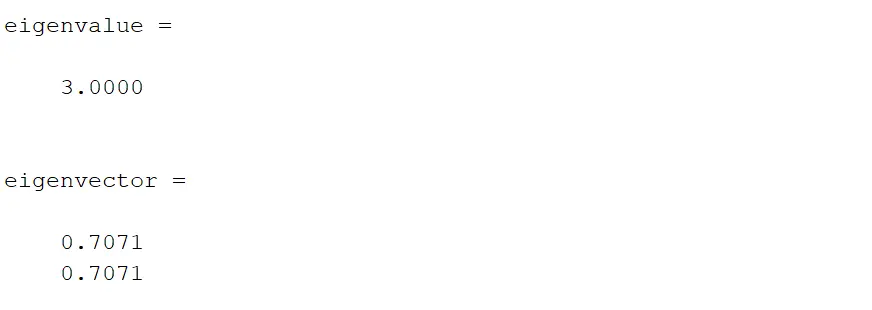
[eigenvalue, eigenvector] = power_iteration(A, tolerance, max_iterations)

In this example, we start by defining our matrix A, a simple 2x2 matrix in this case. This matrix represents the linear transformation under consideration, and we aim to find its dominant eigenvalue and corresponding eigenvector.

Next, we set the convergence tolerance and maximum iterations. These parameters control the behavior of the Power Iteration Method, ensuring that the algorithm converges to accurate results without unnecessary computational overhead.

The convergence tolerance specifies the level of precision we require, while the maximum iterations limit the number of iterations to prevent infinite loops.

We then call the power_iteration function with A, tolerance, and max_iterations as arguments. Inside the power_iteration function, the Power Iteration Method is implemented.

This method involves iteratively applying the matrix A to an initial guess for the eigenvector, normalizing the resulting vector, and repeating the process until convergence. The dominant eigenvalue and eigenvector emerge as the method converges.

Finally, the computed dominant eigenvalue is stored in the variable eigenvalue, and the corresponding eigenvector is stored in the variable eigenvector.

Output:

The Power Iteration Method provides a simple yet effective approach for finding eigenvalues and eigenvectors of matrices, particularly for large sparse matrices.

How to Find the Eigenvector of a Specific Eigenvalue in MATLAB Using Inverse Iteration

Another approach to finding an eigenvector corresponding to a specific eigenvalue is by employing the inverse iteration method. This method involves iterating a sequence of matrix-vector multiplications using the inverse of the matrix until convergence to the desired eigenvector.

The syntax for implementing this method in MATLAB is as follows:

[eigenvector] = inverse_iteration(A, eigenvalue, tolerance, max_iterations);

Here, A is the matrix for which we want to find the eigenvector, eigenvalue is the specific eigenvalue of interest, tolerance specifies the convergence criterion, and max_iterations limits the number of iterations.

Here’s a simplified overview of the inverse iteration method:

Here’s a simple implementation of the inverse iteration algorithm:

function eigenvector = inverse_iteration(A, desired_eigenvalue, tolerance, max_iterations)
    % Initialize the eigenvector guess
    v = randn(size(A, 1), 1);

    % Shift the matrix
    A_shifted = A - desired_eigenvalue * eye(size(A));

    % Iterate until convergence or maximum iterations are reached
    for iter = 1:max_iterations
        % Solve linear system (A - desired_eigenvalue * I) * x = v
        x = A_shifted \ v;

        % Normalize the vector
        eigenvector = x / norm(x);

        % Check for convergence
        if norm(A * eigenvector - desired_eigenvalue * eigenvector) < tolerance
            break;
        end
    end
end

Example: Using Inverse Iteration to Find an Eigenvector Corresponding to a Specific Eigenvalue

Let’s illustrate the Inverse Iteration Method with an example:

% Define the matrix
A = [1 2; 2 1];
desired_eigenvalue = 3;

% Set convergence tolerance and maximum iterations
tolerance = 1e-6;
max_iterations = 100;

% Perform inverse iteration
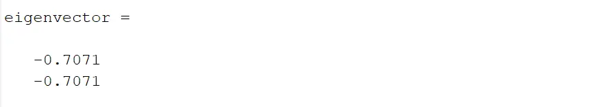
eigenvector = inverse_iteration(A, desired_eigenvalue, tolerance, max_iterations)

In this example, we began by defining our matrix A, a 2x2 matrix in this case, representing the linear transformation under consideration. Alongside, we specified the eigenvalue desired_eigenvalue for which we aimed to find the corresponding eigenvector.

This eigenvalue represents a characteristic value of the linear transformation that we are interested in exploring further.

Next, we set the convergence tolerance and maximum iterations to control the behavior of the Inverse Iteration Method. These parameters determine the level of precision we require in estimating the eigenvector and prevent excessive computational iterations that may lead to inefficiency or divergence.

Subsequently, we called the inverse_iteration function with A, desired_eigenvalue, tolerance, and max_iterations as arguments. Within the inverse_iteration function, the Inverse Iteration Method was implemented.

This method involves iteratively applying the inverse of matrix A to an initial guess for the eigenvector, normalizing the resulting vector, and repeating the process until convergence to the desired eigenvector. By adjusting the convergence tolerance and maximum iterations, we ensured accurate results without excessive computational effort.

Finally, the computed eigenvector was stored in the variable eigenvector.

Output:

Conclusion

MATLAB provides powerful methods for finding eigenvalues and eigenvectors of matrices, including the built-in eig() function, the power iteration method, and the inverse iteration method. These methods enable researchers and engineers to analyze and manipulate linear systems effectively, gaining valuable insights into their behavior and properties.

Whether solving numerical computations, stability analysis, or control systems, MATLAB’s tools empower users to tackle a wide range of mathematical problems involving eigenvalues and eigenvectors with confidence and precision.