How to Draw a Slope Field in MATLAB

1. Understanding Slope Fields
2. Setting Up Your MATLAB Environment
3. Customizing the Slope Field
4. Adding Solution Curves
5. Conclusion
6. FAQ

Creating slope fields for first-order ordinary differential equations is a crucial skill in understanding the behavior of differential equations.

In this tutorial, we will guide you through the steps needed to draw a slope field in MATLAB. Whether you’re a student, educator, or just someone interested in mathematics, this guide will help you visualize the solutions to differential equations effectively. By the end of this tutorial, you will be equipped with the knowledge to create slope fields for various equations, enhancing your understanding of dynamics in mathematical modeling. Let’s dive into the world of MATLAB and explore how to create these informative visualizations.

Understanding Slope Fields

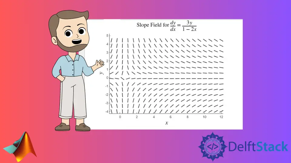
Before we jump into the coding aspect, let’s clarify what a slope field is. A slope field, or direction field, is a graphical representation of the solutions to a first-order differential equation. Each point in the field has a small line segment that represents the slope of the solution curve at that point. This visual tool helps in understanding the behavior of solutions without solving the differential equation analytically.

In MATLAB, we can easily create slope fields using vector fields. The process involves defining a function that describes the differential equation and then plotting the slope field using MATLAB’s built-in functions.

Setting Up Your MATLAB Environment

To get started, ensure you have MATLAB installed on your system. Open MATLAB and create a new script where you can write your code. The following example demonstrates how to create a slope field for the differential equation dy/dx = x - y.

 matlabCopy[x, y] = meshgrid(-5:0.5:5, -5:0.5:5);
dy = x - y;
dx = ones(size(dy));
quiver(x, y, dx, dy);
axis tight;
xlabel('x-axis');
ylabel('y-axis');
title('Slope Field for dy/dx = x - y');

Output:

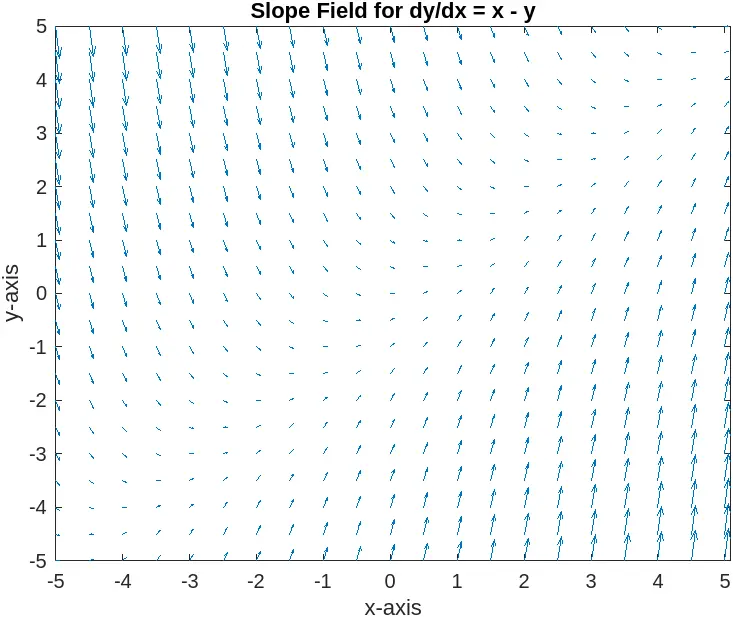
In this code, we first create a grid of points using meshgrid, which generates matrices for the x and y coordinates. The slope of the differential equation is defined by dy = x - y, and dx is set to 1 for uniformity. The quiver function then plots the slope field by drawing arrows at each grid point, indicating the direction of the solution curves. The axis is tightened for better visualization, and labels are added to the x and y axes along with a title for clarity.

Customizing the Slope Field

Now that you have a basic slope field, you may want to customize it further. For instance, you can change the range of x and y values, adjust the density of the arrows, or modify the appearance of the plot. The following example demonstrates how to customize the slope field for the same equation.

 matlabCopy[x, y] = meshgrid(-10:1:10, -10:1:10);
dy = x - y;
dx = ones(size(dy));
figure;
quiver(x, y, dx, dy, 'r');
axis equal;
xlabel('x-axis');
ylabel('y-axis');
title('Customized Slope Field for dy/dx = x - y');

Output:

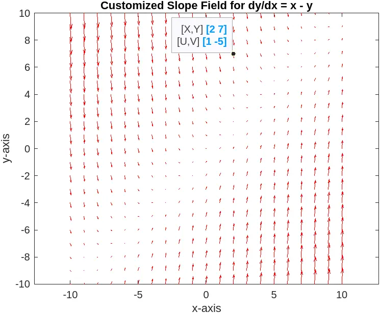
In this customized example, we expanded the range of the grid to -10 to 10 and changed the spacing between the arrows to 1 unit. The color of the arrows is set to red for better visibility. The axis equal command ensures that the scaling of the axes is equal, providing a more accurate representation of the slope field. These adjustments can significantly enhance the clarity and effectiveness of your slope field.

Adding Solution Curves

To further enrich your slope field, you can overlay solution curves. This addition helps visualize how the solutions behave in relation to the slope field. Here’s how you can do that in MATLAB.

 matlabCopy[x, y] = meshgrid(-5:0.5:5, -5:0.5:5);
dy = x - y;
dx = ones(size(dy));
figure;
quiver(x, y, dx, dy);
hold on;

% Define a range of initial conditions for solution curves
for y0 = -4:1:4
    [t, sol] = ode45(@(t, y) t - y, [0 5], y0);
    plot(t, sol, 'LineWidth', 2);
end

axis tight;
xlabel('x-axis');
ylabel('y-axis');
title('Slope Field with Solution Curves for dy/dx = x - y');
hold off;

In this code, we again create the slope field using quiver. The ode45 function is then used to compute the solution curves for various initial conditions (y0). A loop allows us to plot multiple solution curves on the same graph, enhancing our understanding of how the solutions relate to the slope field. The hold on command ensures that both the slope field and the solution curves are displayed together.

Conclusion

Drawing slope fields in MATLAB is a powerful way to visualize the solutions of first-order ordinary differential equations. By following the steps outlined in this tutorial, you can create, customize, and enhance slope fields for various differential equations. This visualization not only aids in understanding the behavior of solutions but also provides insights into the dynamics of mathematical models. With practice, you’ll be able to use these techniques effectively in your studies or research.

FAQ

1. What is a slope field?
   A slope field is a graphical representation of the solutions to a first-order differential equation, showing the slope of the solution curves at various points.

2. How do I create a slope field in MATLAB?
   You can create a slope field in MATLAB using the quiver function, which plots arrows representing the slope defined by your differential equation.

3. Can I customize the slope field in MATLAB?
   Yes, you can customize the slope field by changing the range of x and y values, adjusting the density of arrows, and modifying colors and labels.

4. How do I add solution curves to a slope field?
   You can overlay solution curves on a slope field by using MATLAB’s ode45 function to compute solutions for different initial conditions and then plotting these curves.

5. What are the benefits of using slope fields?
   Slope fields help visualize the behavior of solutions to differential equations, making it easier to understand their dynamics without solving them analytically.