How to Plot Root Locus in MATLAB

1. Understanding Root Locus
2. Setting Up the Transfer Function
3. Customizing the Root Locus Plot
4. Analyzing the Root Locus
5. Conclusion
6. FAQ

Root locus is a powerful tool in control system design, allowing engineers to visualize how the roots of a system’s characteristic equation change with varying feedback gain. MATLAB provides an intuitive function called rlocus() to facilitate this process.

In this article, we will explore how to plot root locus in MATLAB, breaking down the steps and providing clear examples. Whether you’re a student or a seasoned engineer, this guide will enhance your understanding of dynamic systems and control theory. Let’s dive into the world of root locus and see how MATLAB can simplify our analysis.

Understanding Root Locus

Root locus is a graphical method used to study how the roots of a transfer function move in the complex plane as a particular parameter, typically gain, varies. The root locus plot provides vital insights into system stability and transient response. By plotting the root locus, engineers can determine the gain values that yield desired performance characteristics.

In MATLAB, the rlocus() function is the primary tool used for generating these plots. This function allows for straightforward visualization of the root locus for continuous-time linear systems. To get started, you will need to define your system’s transfer function using the Control System Toolbox.

Setting Up the Transfer Function

Before we can plot the root locus, we need to define a transfer function in MATLAB. This can be done using the tf() function, which creates a transfer function model. Below is an example of how to define a simple first-order system and plot its root locus.

num = [2 5 1]; 
den = [1, 2, 3]; 
sys = tf(num, den); 
rlocus(sys); 

In this example, we define a transfer function with a numerator of 1 and a denominator of s² + 2s + 1. The tf() function creates the transfer function model, which we then pass to rlocus(). The plot will display the root locus for the defined system, showing how the poles shift in the s-plane as gain varies.

Output:

This simple setup allows you to visualize the dynamic behavior of the system as feedback gain changes. By analyzing the plot, you can make informed decisions about system stability and performance.

Customizing the Root Locus Plot

MATLAB’s rlocus() function offers several options for customization to enhance the clarity and aesthetics of your plot. You can modify the axis limits, add grid lines, and even change the color and style of the plot. Here’s how you can customize your root locus plot:

num = [1]; 
den = [1, 2, 1]; 
sys = tf(num, den); 
rlocus(sys); 
title('Customized Root Locus');
grid on; 
xlim([-3 1]); 
ylim([-2 2]);

In this code snippet, we’ve added a title and enabled the grid for better visibility. The xlim() and ylim() functions define the limits for the x-axis and y-axis, respectively. This customization helps in focusing on specific regions of the root locus, making it easier to analyze critical points.

Output:

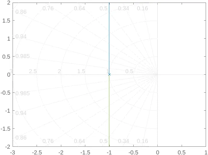
Customizing your plot can significantly improve the interpretability of your results, especially when presenting to stakeholders or during academic discussions.

Analyzing the Root Locus

Once you have your root locus plotted, the next step is to analyze the results. The root locus provides valuable information about system stability. The location of the poles in the s-plane indicates whether the system is stable or unstable. For instance, if all poles lie in the left half-plane, the system is stable. Conversely, poles in the right half-plane indicate instability.

To analyze the root locus effectively, consider the following:

1. Gain Values: Identify the gain values that correspond to desired pole locations.
2. Damping Ratio: Assess the damping ratio from the pole locations to evaluate transient response characteristics.
3. Natural Frequency: Determine the natural frequency of the system from the pole locations for further insights into system behavior.

By understanding the implications of your root locus, you can make informed design decisions, such as adjusting feedback gain to achieve desired performance metrics.

Output:

Analysis of the root locus reveals stability characteristics of the system.

Conclusion

Plotting the root locus in MATLAB is a straightforward yet powerful technique for analyzing dynamic systems. By utilizing the rlocus() function, you can create informative visualizations that help in understanding system behavior under varying conditions. Customizations further enhance clarity, enabling you to focus on critical aspects of your analysis. As you become more familiar with root locus techniques, you’ll find them indispensable for control system design and stability analysis. Embrace the power of MATLAB, and take your control systems knowledge to new heights.

FAQ

1. What is root locus in control systems?
   Root locus is a graphical method used to analyze how the roots of a system’s characteristic equation change with varying feedback gain.

2. How do I plot root locus in MATLAB?
   You can plot root locus in MATLAB using the rlocus() function after defining your system’s transfer function with the tf() function.

3. What does the root locus plot indicate about system stability?
   The location of the poles in the root locus plot indicates whether a system is stable or unstable. Poles in the left half-plane signify stability, while those in the right half-plane indicate instability.

4. Can I customize my root locus plot in MATLAB?
   Yes, MATLAB allows for various customizations, such as adjusting axis limits, adding grid lines, and changing plot colors and styles.

5. How can I analyze the root locus results?
   You can analyze the root locus by examining gain values, damping ratios, and natural frequencies derived from the pole locations.