The meshgrid() Function in MATLAB

1. Understanding the meshgrid() Function
2. Creating a Simple Grid with meshgrid()
3. Visualizing the Grid with meshgrid()
4. Advanced Applications of meshgrid()
5. Conclusion
6. FAQ

Creating grids is a fundamental task in many mathematical and engineering applications, and the meshgrid() function in MATLAB makes this process seamless. Whether you’re dealing with surface plots, simulations, or data visualization, understanding how to utilize meshgrid() can significantly enhance your workflow. This powerful function generates a grid of coordinates based on two input vectors, enabling you to evaluate functions over a specified range.

In this article, we will dive deep into the meshgrid() function, exploring its syntax, practical applications, and providing clear examples to help you grasp its utility. By the end, you’ll be well-equipped to leverage this function in your own MATLAB projects.

Understanding the meshgrid() Function

The meshgrid() function takes two input vectors, typically representing the x and y coordinates, and produces two 2D matrices. Each matrix corresponds to the x and y coordinates of a grid that covers the specified ranges. This is particularly useful for evaluating functions of two variables, as it allows you to create a full grid of points over which you can compute values.

The syntax for the meshgrid() function is straightforward:

[X, Y] = meshgrid(x, y);

Here, x and y are the input vectors, while X and Y are the resulting matrices. The output matrices will have dimensions that correspond to the lengths of the input vectors, allowing for easy manipulation and evaluation.

Creating a Simple Grid with meshgrid()

To illustrate the use of meshgrid(), let’s start with a simple example. Suppose we want to create a grid for the x-coordinates ranging from -5 to 5 and y-coordinates from -5 to 5. Here’s how you can do that:

x = -5:1:5;
y = -5:1:5;
[X, Y] = meshgrid(x, y);

Output:

X =

    -5    -4    -3    -2    -1     0     1     2     3     4     5
    -5    -4    -3    -2    -1     0     1     2     3     4     5
    -5    -4    -3    -2    -1     0     1     2     3     4     5
    -5    -4    -3    -2    -1     0     1     2     3     4     5
    -5    -4    -3    -2    -1     0     1     2     3     4     5
    -5    -4    -3    -2    -1     0     1     2     3     4     5
    -5    -4    -3    -2    -1     0     1     2     3     4     5
    -5    -4    -3    -2    -1     0     1     2     3     4     5
    -5    -4    -3    -2    -1     0     1     2     3     4     5
    -5    -4    -3    -2    -1     0     1     2     3     4     5
    -5    -4    -3    -2    -1     0     1     2     3     4     5

Y =

    -5    -5    -5    -5    -5    -5    -5    -5    -5    -5    -5
    -4    -4    -4    -4    -4    -4    -4    -4    -4    -4    -4
    -3    -3    -3    -3    -3    -3    -3    -3    -3    -3    -3
    -2    -2    -2    -2    -2    -2    -2    -2    -2    -2    -2
    -1    -1    -1    -1    -1    -1    -1    -1    -1    -1    -1
     0     0     0     0     0     0     0     0     0     0     0
     1     1     1     1     1     1     1     1     1     1     1
     2     2     2     2     2     2     2     2     2     2     2
     3     3     3     3     3     3     3     3     3     3     3
     4     4     4     4     4     4     4     4     4     4     4
     5     5     5     5     5     5     5     5     5     5     5

In this example, we defined the x-coordinates and y-coordinates as vectors ranging from -5 to 5. After executing meshgrid(), we obtained matrices X and Y. Each element of X corresponds to the x-coordinate of the grid, while Y contains the respective y-coordinates. This grid is now ready for further computations, such as evaluating functions or creating plots.

Visualizing the Grid with meshgrid()

Once you have created your grid using meshgrid(), visualizing it can provide insights into the data or functions you are working with. Let’s create a 3D surface plot based on the grid we generated earlier. For this example, we will evaluate the function z = x^2 + y^2.

Z = X.^2 + Y.^2;
surf(X, Y, Z);
xlabel('X-axis');
ylabel('Y-axis');
zlabel('Z-axis');
title('Surface Plot of z = x^2 + y^2');

Output:

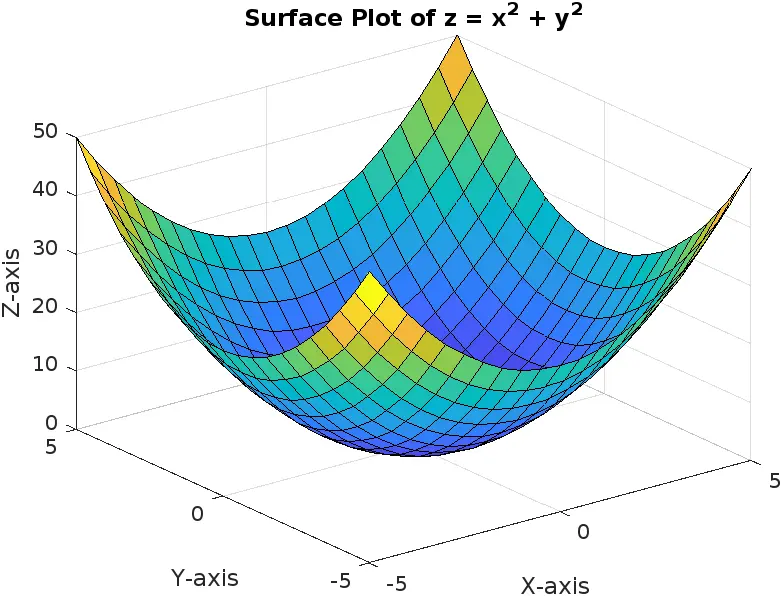
In this code snippet, we first calculate the z-values using the formula Z = X.^2 + Y.^2. The .^ operator is used to perform element-wise exponentiation, which is essential when working with matrices. After computing the z-values, we use the surf() function to create a surface plot. The labels and title enhance the plot’s clarity, making it easier for viewers to understand the visual representation of the function.

This visualization technique is particularly useful in fields such as engineering, physics, and data science, where understanding the behavior of functions in three dimensions can lead to valuable insights.

Advanced Applications of meshgrid()

The meshgrid() function can also be applied in more advanced scenarios, such as contour plotting or evaluating more complex mathematical functions. For instance, let’s consider a scenario where we want to visualize the contours of the function z = sin(sqrt(x^2 + y^2)). This can be achieved by using the contour() function in MATLAB.

Z = sin(sqrt(X.^2 + Y.^2));
contour(X, Y, Z);
xlabel('X-axis');
ylabel('Y-axis');
title('Contour Plot of z = sin(sqrt(x^2 + y^2))');

Output:

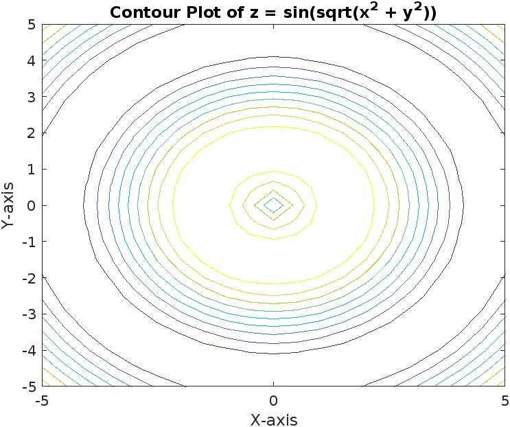
In this example, we compute the z-values using the function Z = sin(sqrt(X.^2 + Y.^2)). The contour() function then creates a contour plot, which provides a different perspective on the function’s behavior. Contour plots are particularly useful for visualizing levels of a function and can be used in optimization problems or geographical mapping.

By leveraging the meshgrid() function in conjunction with plotting functions like surf() and contour(), you can create a variety of visual representations that make complex data more interpretable and actionable.

Conclusion

The meshgrid() function in MATLAB is an invaluable tool for creating grids of coordinates, which can be utilized in various mathematical and engineering contexts. From simple grid creation to advanced visualizations, mastering this function can greatly enhance your ability to work with multidimensional data. Whether you’re plotting surfaces, contours, or evaluating functions, understanding how to effectively use meshgrid() will undoubtedly improve your MATLAB programming skills. So go ahead, experiment with this powerful function, and unlock new possibilities in your projects.

FAQ

1. What is the purpose of the meshgrid() function in MATLAB?
   The meshgrid() function creates a grid of coordinates based on two input vectors, allowing for the evaluation of functions over a specified range.

2. Can I use meshgrid() for 3D plotting?
   Yes, meshgrid() is often used in conjunction with functions like surf() and mesh() to create 3D plots based on the generated grid.

3. What types of visualizations can I create using meshgrid()?
   You can create various visualizations, including surface plots, contour plots, and even heatmaps, by evaluating functions over the grid generated by meshgrid().

4. Is meshgrid() limited to two dimensions?
   Yes, meshgrid() primarily works with two input vectors to create 2D grids. However, you can extend its concepts to higher dimensions with additional coding.

5. How does meshgrid() handle non-uniform spacing in vectors?
   meshgrid() will create grids based on the exact values of the input vectors, so non-uniform spacing will be preserved in the output matrices.