MATLAB Dirac Delta Function

1. Plotting the Dirac Delta Function Using plot()
2. Visualizing the Dirac Delta Function Using stem()
3. Using the dirac() Function for Accurate Representation
4. Conclusion
5. FAQ

The Dirac delta function is a fascinating mathematical concept often used in engineering and physics. It serves as an idealized point source, providing a way to model impulses in systems. MATLAB, a powerful tool for numerical computing, allows users to visualize this function effectively.

In this article, we will explore how to plot the Dirac delta function using the plot(), stem(), and dirac() functions in MATLAB. Whether you’re a student or a professional, understanding how to manipulate and visualize this function can significantly enhance your analytical skills. Let’s dive in and see how we can achieve this, complete with code examples and explanations.

Plotting the Dirac Delta Function Using plot()

The plot() function in MATLAB is a versatile tool for creating continuous line graphs. However, since the Dirac delta function is not a traditional function but rather a distribution, it requires a special approach for visualization. Here’s how you can use the plot() function to represent the Dirac delta function.

x = -5:0.01:5;
y = zeros(size(x));
y(x==0) = 1; % Assigning a value at x = 0

figure;
plot(x, y, 'LineWidth', 2);
title('Dirac Delta Function using plot()');
xlabel('x');
ylabel('Amplitude');
grid on;

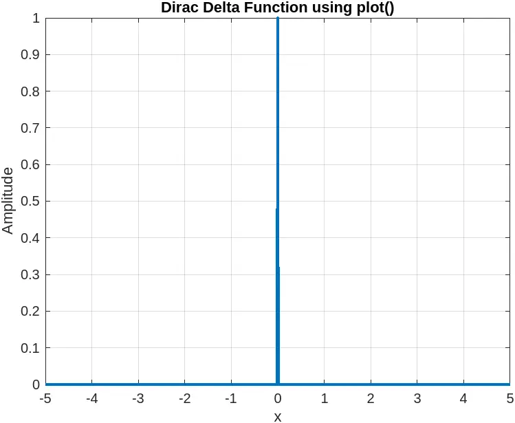
In this code, we create a vector x that spans from -5 to 5. We initialize a vector y of the same size, filled with zeros. The line y(x==0) = 1; assigns the value of 1 at the point where x is zero, effectively simulating the Dirac delta function. The plot() function then generates a line plot, which visually represents this impulse at the origin. The grid enhances readability, while the title and labels provide context to the graph.

This method gives a clear visual representation of the Dirac delta function, making it easier to understand its behavior in the context of systems and signals.

Visualizing the Dirac Delta Function Using stem()

The stem() function is another effective way to visualize discrete data in MATLAB. It provides a clear representation of the Dirac delta function, particularly useful for illustrating its impulse nature. Let’s see how to implement this.

x = -5:1:5;
y = zeros(size(x));
y(x==0) = 1; 

figure;
stem(x, y, 'filled');
title('Dirac Delta Function using stem()');
xlabel('x');
ylabel('Amplitude');
grid on;

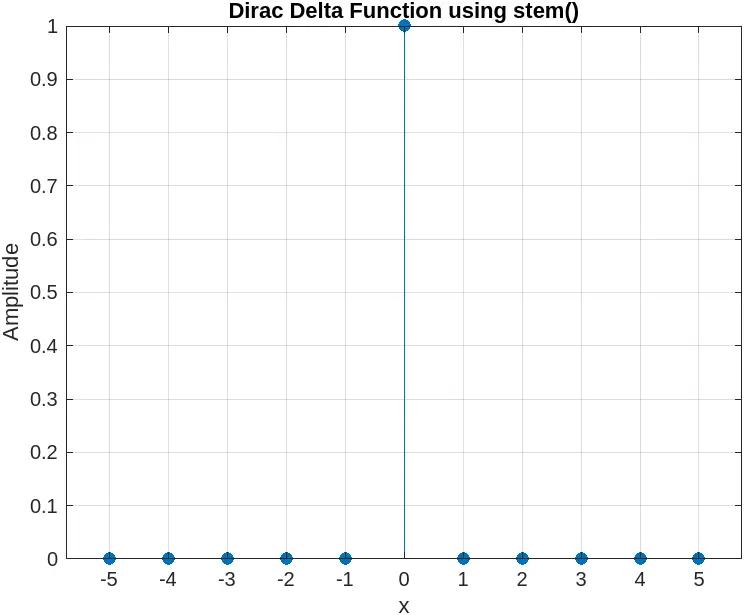
In this example, we define a vector x with integer steps from -5 to 5. Similar to the previous method, we create a y vector filled with zeros and set y(x==0) = 1; to indicate the impulse at the origin. The stem() function then generates a stem plot, which is particularly effective for illustrating discrete functions and impulses. The filled markers provide a clear visual cue, enhancing the understanding of the function’s behavior.

Using the stem() function allows for a more discrete representation of the Dirac delta function, which can be particularly useful in digital signal processing contexts.

Using the dirac() Function for Accurate Representation

MATLAB also offers a built-in dirac() function that directly represents the Dirac delta function. This method is the most straightforward and accurate way to visualize the Dirac delta function. Here’s how to use it.

syms x;
f = dirac(x); % Define Dirac delta function

fplot(f, [-5 5], 'LineWidth', 2);
title('Dirac Delta Function using dirac()');
xlabel('x');
ylabel('Amplitude');
grid on;

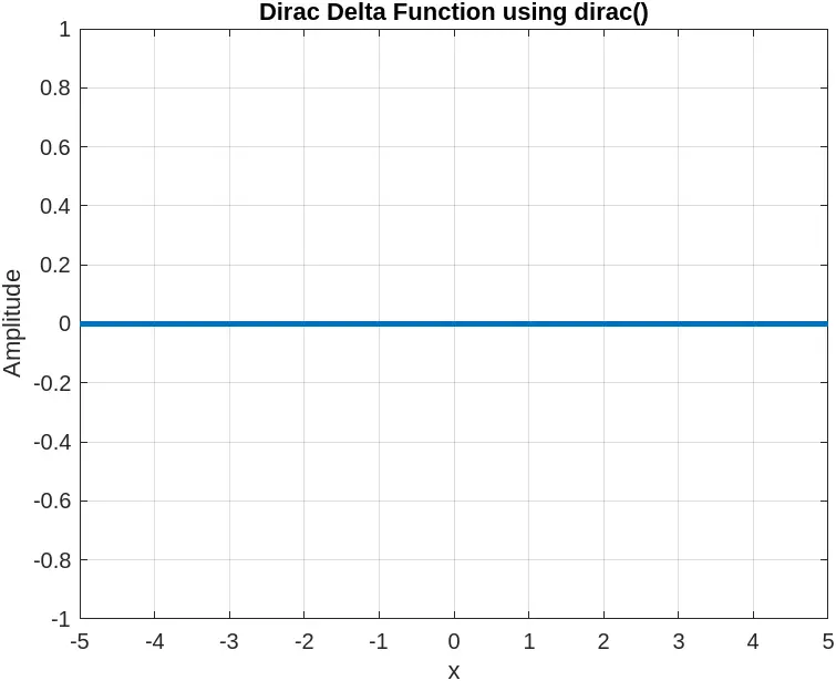
In this code snippet, we leverage symbolic computation by using the syms command to define x as a symbolic variable. The dirac(x) function creates the Dirac delta function symbolically. The fplot() function then plots this symbolic function over the specified range from -5 to 5. This method provides a mathematically accurate representation of the Dirac delta function, ensuring that the impulse is correctly depicted.

Using the dirac() function is the most efficient way to plot the Dirac delta function in MATLAB, especially for those looking for precision and ease of use.

Conclusion

In summary, plotting the Dirac delta function in MATLAB can be accomplished using various methods, including the plot(), stem(), and dirac() functions. Each method offers unique advantages, whether you prefer a continuous representation, a discrete visualization, or a mathematically accurate plot. Understanding how to visualize this function is essential for anyone working in fields like signal processing, control systems, or physics. By mastering these techniques, you can deepen your insights into impulse responses and their applications in real-world systems.

FAQ

1. what is the Dirac delta function?
   The Dirac delta function is a mathematical construct that represents an idealized point source or impulse in a system.

2. how is the Dirac delta function used in engineering?
   It is used to model impulses, such as in signal processing and control systems, allowing engineers to analyze system responses.

3. can I use the dirac() function in MATLAB without symbolic math?
   No, the dirac() function requires the symbolic math toolbox to work effectively.

4. what are the differences between plot() and stem() when visualizing the Dirac delta function?
   The plot() function provides a continuous representation, while the stem() function offers a discrete view, making it more suitable for illustrating impulses.

5. is it necessary to use MATLAB to plot the Dirac delta function?
   While MATLAB is a powerful tool for this purpose, other programming environments like Python can also visualize the Dirac delta function effectively.