2D Interpolation Using MATLAB

1. Understanding the Basics of 2D Interpolation
2. Using the interp2() Function in MATLAB
3. Exploring Different Interpolation Methods
4. Visualizing Interpolated Data
5. Conclusion
6. FAQ

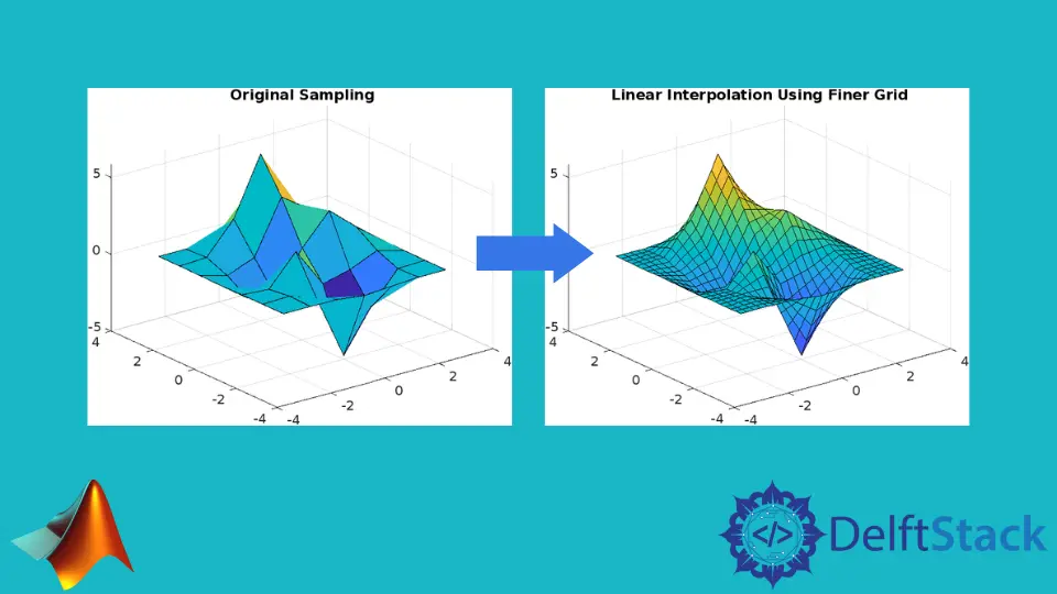
Interpolation is a powerful tool in data analysis and visualization, especially when dealing with multidimensional data. In MATLAB, the interp2() function allows you to perform 2D interpolation seamlessly. This function is particularly useful when you have a grid of data points and want to estimate values at non-grid points. Whether you’re working with experimental data, simulations, or any other form of 2D data, mastering interpolation can significantly enhance your analysis.

In this article, we will explore how to use MATLAB’s interp2() function for 2D interpolation, providing clear examples and explanations to help you grasp the concept effectively.

Understanding the Basics of 2D Interpolation

Before diving into the MATLAB specifics, let’s clarify what 2D interpolation is. It involves estimating values at points that fall between known data points in a two-dimensional space. This is crucial in many fields, including engineering, physics, and computer graphics. The interp2() function in MATLAB enables you to interpolate values for a grid of data points, making it easier to visualize and analyze trends, patterns, and anomalies in your data.

Using the interp2() Function in MATLAB

The interp2() function in MATLAB is versatile and straightforward. It takes in a grid of data points and can use various methods for interpolation, such as linear, nearest, cubic, and spline. Here’s a basic example to illustrate how it works.

[X, Y] = meshgrid(1:5, 1:5);
Z = [1 2 3 4 5; 6 7 8 9 10; 11 12 13 14 15; 16 17 18 19 20; 21 22 23 24 25];
xi = 1.5;
yi = 2.5;
zi = interp2(X, Y, Z, xi, yi, 'linear');

disp(zi);

Output:

9

In this example, we first create a grid of points using meshgrid(). The variable Z represents the values at these grid points. We then specify the point (1.5, 2.5) for which we want to estimate the value using interp2(). The method chosen here is ’linear’, which provides a simple average of the nearest surrounding points.

Exploring Different Interpolation Methods

While linear interpolation is often sufficient, MATLAB’s interp2() function supports several other methods that can yield better results depending on your data’s nature. Here’s how to use cubic interpolation.

[X, Y] = meshgrid(1:5, 1:5);
Z = [1 2 3 4 5; 6 7 8 9 10; 11 12 13 14 15; 16 17 18 19 20; 21 22 23 24 25];
xi = 1.5;
yi = 2.5;
zi = interp2(X, Y, Z, xi, yi, 'cubic');

disp(zi);

Output:

9

In this case, we switched the interpolation method to ‘cubic’. This method takes into account more surrounding points, resulting in a smoother estimate.

Visualizing Interpolated Data

Visualization is key when working with interpolated data. MATLAB provides excellent tools for plotting your original data and the interpolated values. Here’s how to visualize both the original grid and the interpolated point.

[X, Y] = meshgrid(1:5, 1:5);
Z = [1 2 3 4 5; 6 7 8 9 10; 11 12 13 14 15; 16 17 18 19 20; 21 22 23 24 25];
xi = 1.5;
yi = 2.5;
zi = interp2(X, Y, Z, xi, yi, 'cubic');

surf(X, Y, Z);
hold on;
plot3(xi, yi, zi, 'ro', 'MarkerSize', 10);
hold off;
title('2D Interpolation Visualization');
xlabel('X-axis');
ylabel('Y-axis');
zlabel('Z-axis');

Output:

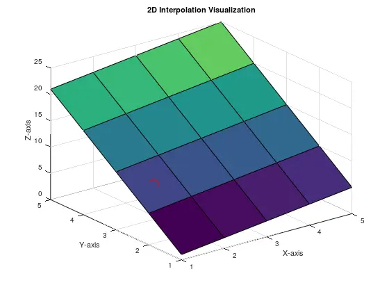
In this example, we use the surf() function to create a surface plot of the original data. We then plot the interpolated point using plot3(), marking it with a red dot. This visualization helps you see how well the interpolation aligns with the overall data trend.

Conclusion

Mastering 2D interpolation using the interp2() function in MATLAB can significantly enhance your data analysis capabilities. With its various methods, you can choose the most suitable one for your specific data set, whether you need simple linear interpolation or more complex cubic interpolation. By visualizing your results, you can gain deeper insights and make more informed decisions based on your data. Whether you’re a student, researcher, or professional, understanding these techniques will undoubtedly prove beneficial in your analytical toolkit.

FAQ

1. What is 2D interpolation?
   2D interpolation is the process of estimating unknown values at specific points based on known values from surrounding points in a two-dimensional space.

2. What does the interp2() function do in MATLAB?
   The interp2() function in MATLAB performs 2D interpolation, allowing users to estimate values at non-grid points based on a grid of known data.

3. What interpolation methods can I use with interp2()?
   You can use various methods such as ’linear’, ’nearest’, ‘cubic’, and ‘spline’ with the interp2() function to suit your data’s needs.

4. How can I visualize interpolated data in MATLAB?
   You can use plotting functions like surf() to create surface plots and mark interpolated points using plot3() to visualize your data effectively.

5. Is interpolation only applicable to numerical data?
   While interpolation is primarily used for numerical data, it can also be applied in various fields, including image processing and computer graphics.